LLM Optimization
Large Model Optimization on PyTorch

PyTorch 2.0

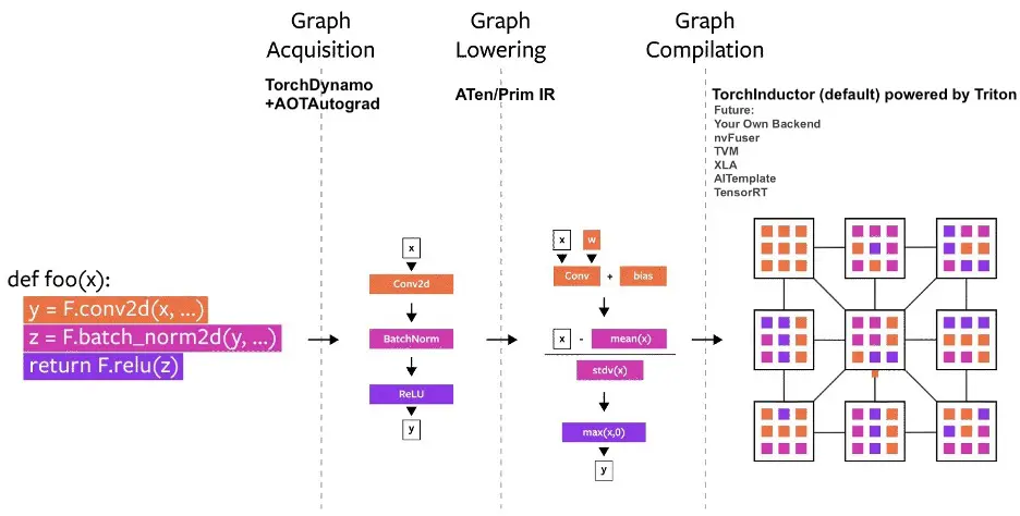
torch.compile
opt_module = torch.compile(module)Depending on the model and the GPU, torch.compile() yields up to 30% speed-up during inference. To use torch.compile(), simply install any version of torch above 2.0.
Underpinning torch.compile are new technologies – TorchDynamo, AOTAutograd, PrimTorch and TorchInductor.
- TorchDynamo captures PyTorch programs safely using Python Frame Evaluation Hooks and is a significant innovation that was a result of 5 years of our R&D into safe graph capture
- AOTAutograd overloads PyTorch’s autograd engine as a tracing autodiff for generating ahead-of-time backward traces.
- PrimTorch canonicalizes ~2000+ PyTorch operators down to a closed set of ~250 primitive operators that developers can target to build a complete PyTorch backend. This substantially lowers the barrier of writing a PyTorch feature or backend.
- TorchInductor is a deep learning compiler that generates fast code for multiple accelerators and backends. For NVIDIA and AMD GPUs, it uses OpenAI Triton as a key building block.
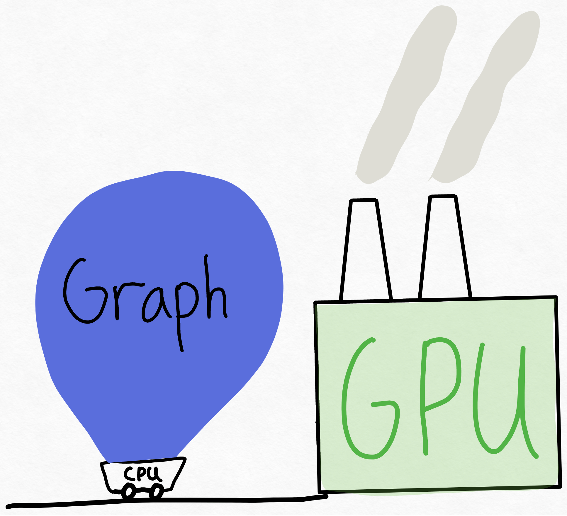
Imagine the GPU as this super massive factory with a ridiculous amount of compute available. Then, imagine the CPU as some messenger shuttling instructions back and forth to the GPU. Remember, in large scale deep learning systems, the GPU is responsible for doing 100% of the work! In such systems, the only role of the CPU is to tell the GPU what work it should be doing.
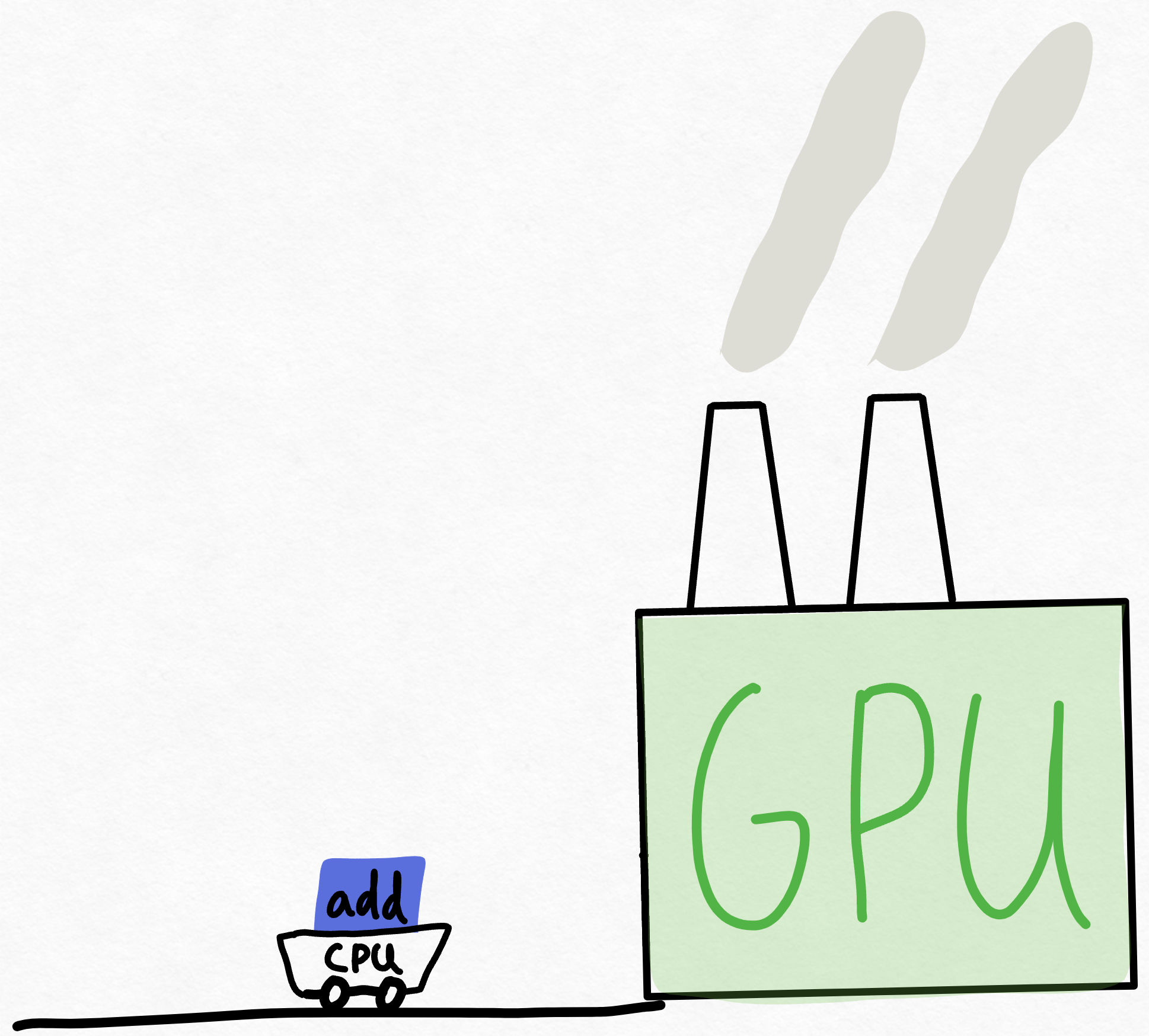
So, the CPU runs over and tells the GPU to do an “add”, but by the time the CPU can give the GPU another chunk of work, the GPU has long finished the previous chunk of work.
Despite the fact that the GPU needs to perform thousands of computations while the CPU only needs to do orchestration work, this is surprisingly common! There’s a variety of reasons for this, ranging from the fact that the CPU is likely running some single-threaded Python to the fact that GPUs are just incredibly fast nowadays.
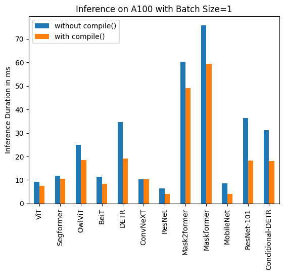
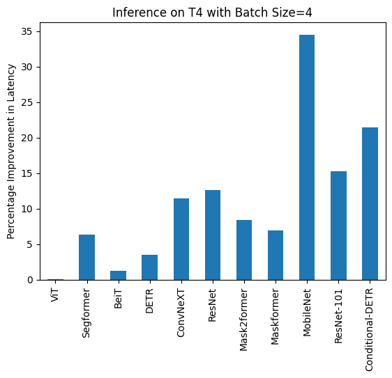
Some Benchmarks
A100
| Task/Model | Batch Size | torch 2.0 -no compile | torch 2.0 -compile |
|---|---|---|---|
| Image Classification/ConvNeXT | Unbatched | 11.758 | 7.335 |
| Image Classification/ConvNeXT | 4 | 23.171 | 21.490 |
| Image Classification/ResNet | Unbatched | 7.435 | 3.801 |
| Image Classification/ResNet | 4 | 7.261 | 2.187 |
| Object Detection/Conditional-DETR | Unbatched | 32.823 | 11.627 |
| Object Detection/Conditional-DETR | 4 | 50.622 | 33.831 |
| Image Segmentation/MobileNet | Unbatched | 9.869 | 4.244 |
| Image Segmentation/MobileNet | 4 | 14.385 | 7.946 |
T4
| Task/Model | Batch Size | torch 2.0 -no compile | torch 2.0 -compile |
|---|---|---|---|
| Image Classification/ConvNeXT | Unbatched | 32.137 | 31.84 |
| Image Classification/ConvNeXT | 4 | 120.944 | 110.209 |
| Image Classification/ResNet | Unbatched | 9.761 | 7.698 |
| Image Classification/ResNet | 4 | 15.215 | 13.871 |
| Object Detection/Conditional-DETR | Unbatched | 72.150 | 57.660 |
| Object Detection/Conditional-DETR | 4 | 301.494 | 247.543 |
| Image Segmentation/MobileNet | Unbatched | 22.266 | 19.339 |
| Image Segmentation/MobileNet | 4 | 78.311 | 50.983 |
https://pytorch.org/get-started/pytorch-2.0/#user-experience
Usage
# default: optimizes for large models, low compile-time
#          and no extra memory usage
torch.compile(model)

# reduce-overhead: optimizes to reduce the framework overhead
#                and uses some extra memory. Helps speed up small models
torch.compile(model, mode="reduce-overhead")

# max-autotune: optimizes to produce the fastest model,
#               but takes a very long time to compile
torch.compile(model, mode="max-autotune")
We’re going to test torch.compile on google/vit-large-patch32-384
Colab Notebook: https://colab.research.google.com/drive/133DghyCIABxvYsQ5LV7TkqDsXKJMgwtP?usp=sharing
We will be needing pytorch profiler to see what exactly is going on when inferencing
def profile_model(model, image, trace_filename):
    inputs = feature_extractor(images=image, return_tensors="pt")
    inputs = inputs.to(device)
    with profile(
        activities=[ProfilerActivity.CPU, ProfilerActivity.CUDA],
        record_shapes=True,
        with_stack=True
    ) as prof:
        with torch.no_grad():
            model(**inputs)

    print(prof.key_averages().table(sort_by="cuda_time_total", row_limit=10))
    prof.export_chrome_trace(trace_filename)  # Save as .json file
And benchmark the model with
def benchmark_model(model, feature_extractor, image, batch_size):
    inputs = feature_extractor(images=[image for _ in range(batch_size)], return_tensors="pt")
    inputs = inputs.to(device)

    print("🔥 warming up model...")
    with torch.no_grad():
        for _ in range(10):
            _ = model(**inputs)

    print(f"performing benchmark with {batch_size=}")
    durations = []
    for _ in range(10):
        start_time = time.time()
        with torch.no_grad():
            _ = model(**inputs)
        end_time = time.time()
        durations.append((end_time - start_time) * 1000)  # Convert to milliseconds

    avg_duration = sum(durations) / len(durations)
    throughput = (batch_size / avg_duration) * 1000  # images per second

    print(f"Average inference time with {batch_size=}: {avg_duration=:.2f} ms")
    print(f"Model throughput with {batch_size=}: {throughput=:.2f} images/s")

    return avg_duration, throughput
feature_extractor = ViTFeatureExtractor.from_pretrained('google/vit-large-patch32-384')
model = ViTForImageClassification.from_pretrained('google/vit-large-patch32-384')Compiling the model is as simple as
compiled_model = torch.compile(model)torch.compile(model, mode="reduce-overhead")”reduce-overhead” is a mode that reduces the overhead of python with CUDA graphs, useful for small batches. Reduction of overhead can come at the cost of more memory usage, as we will cache the workspace memory required for the invocation so that we do not have to reallocate it on subsequent runs.
RAW Model
------------------------------------------------------- ------------ ------------ ------------ ------------ ------------ ------------ ------------ ------------ ------------ ------------
Name Self CPU % Self CPU CPU total % CPU total CPU time avg Self CUDA Self CUDA % CUDA total CUDA time avg # of Calls
------------------------------------------------------- ------------ ------------ ------------ ------------ ------------ ------------ ------------ ------------ ------------ ------------
aten::linear 2.64% 2.559ms 55.25% 53.458ms 368.676us 0.000us 0.00% 58.653ms 404.503us 145
aten::addmm 40.76% 39.443ms 45.22% 43.760ms 301.793us 50.857ms 86.83% 58.653ms 404.503us 145
volta_sgemm_128x64_tn 0.00% 0.000us 0.00% 0.000us 0.000us 50.685ms 86.53% 50.685ms 351.979us 144
cudaLaunchKernel 13.25% 12.820ms 13.25% 12.820ms 32.872us 7.125ms 12.16% 7.125ms 18.269us 390
cudaOccupancyMaxActiveBlocksPerMultiprocessor 0.53% 511.000us 0.53% 511.000us 1.774us 3.556ms 6.07% 3.556ms 12.347us 288
aten::matmul 1.12% 1.088ms 5.72% 5.539ms 115.396us 0.000us 0.00% 3.535ms 73.646us 48
aten::bmm 1.99% 1.923ms 2.79% 2.703ms 56.312us 3.179ms 5.43% 3.535ms 73.646us 48
aten::conv2d 0.02% 18.000us 4.01% 3.879ms 3.879ms 0.000us 0.00% 2.136ms 2.136ms 1
aten::convolution 0.03% 26.000us 3.99% 3.861ms 3.861ms 0.000us 0.00% 2.136ms 2.136ms 1
aten::_convolution 1.55% 1.498ms 3.96% 3.835ms 3.835ms 0.000us 0.00% 2.136ms 2.136ms 1
------------------------------------------------------- ------------ ------------ ------------ ------------ ------------ ------------ ------------ ------------ ------------ ------------
Self CPU time total: 96.762ms
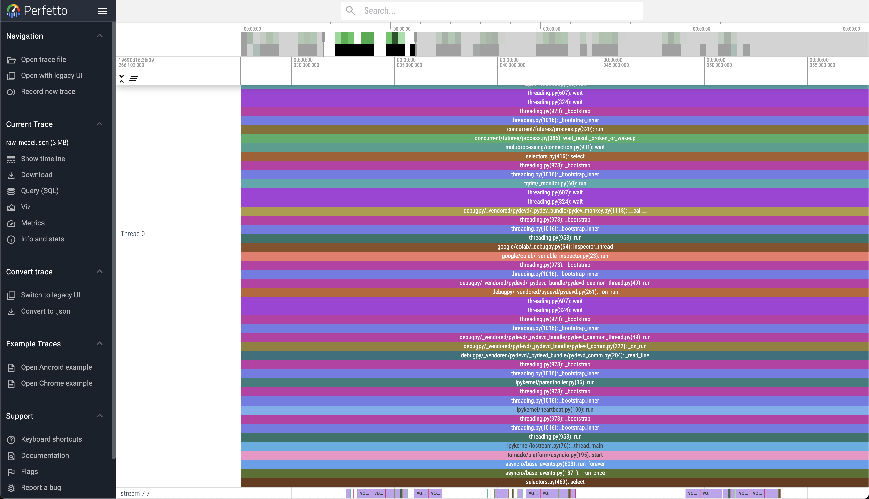
Self CUDA time total: 58.572msThe Trace files .json generated can be viewed at https://ui.perfetto.dev/ or chrome://tracing/
Compiled Model
-------------------------------------------------------  ------------  ------------  ------------  ------------  ------------  ------------  ------------  ------------  ------------  ------------
                                                   Name    Self CPU %      Self CPU   CPU total %     CPU total  CPU time avg     Self CUDA   Self CUDA %    CUDA total  CUDA time avg    # of Calls
-------------------------------------------------------  ------------  ------------  ------------  ------------  ------------  ------------  ------------  ------------  ------------  ------------
                                               aten::mm        10.72%       4.215ms        16.19%       6.368ms      44.222us      49.187ms        86.68%      49.187ms     341.576us           144
                        volta_sgemm_128x32_sliced1x4_tn         0.00%       0.000us         0.00%       0.000us       0.000us      33.034ms        58.21%      33.034ms     275.283us           120
                                  volta_sgemm_128x64_tn         0.00%       0.000us         0.00%       0.000us       0.000us      16.129ms        28.42%      16.129ms     672.042us            24
          aten::_scaled_dot_product_efficient_attention         1.61%     635.000us         7.38%       2.903ms     120.958us       0.000us         0.00%       3.665ms     152.708us            24
                     aten::_efficient_attention_forward         2.04%     803.000us         4.54%       1.787ms      74.458us       3.665ms         6.46%       3.665ms     152.708us            24
fmha_cutlassF_f32_aligned_64x64_rf_sm75(PyTorchMemEf...         0.00%       0.000us         0.00%       0.000us       0.000us       3.665ms         6.46%       3.665ms     152.708us            24
                                      aten::convolution         0.04%      17.000us         0.56%     220.000us     220.000us       0.000us         0.00%       2.125ms       2.125ms             1
                                     aten::_convolution         0.04%      17.000us         0.52%     203.000us     203.000us       0.000us         0.00%       2.125ms       2.125ms             1
                                aten::cudnn_convolution         0.33%     128.000us         0.47%     186.000us     186.000us       2.125ms         3.74%       2.125ms       2.125ms             1
void implicit_convolve_sgemm<float, float, 512, 6, 8...         0.00%       0.000us         0.00%       0.000us       0.000us       2.125ms         3.74%       2.125ms       2.125ms             1
-------------------------------------------------------  ------------  ------------  ------------  ------------  ------------  ------------  ------------  ------------  ------------  ------------
Self CPU time total: 39.321ms
Self CUDA time total: 56.745ms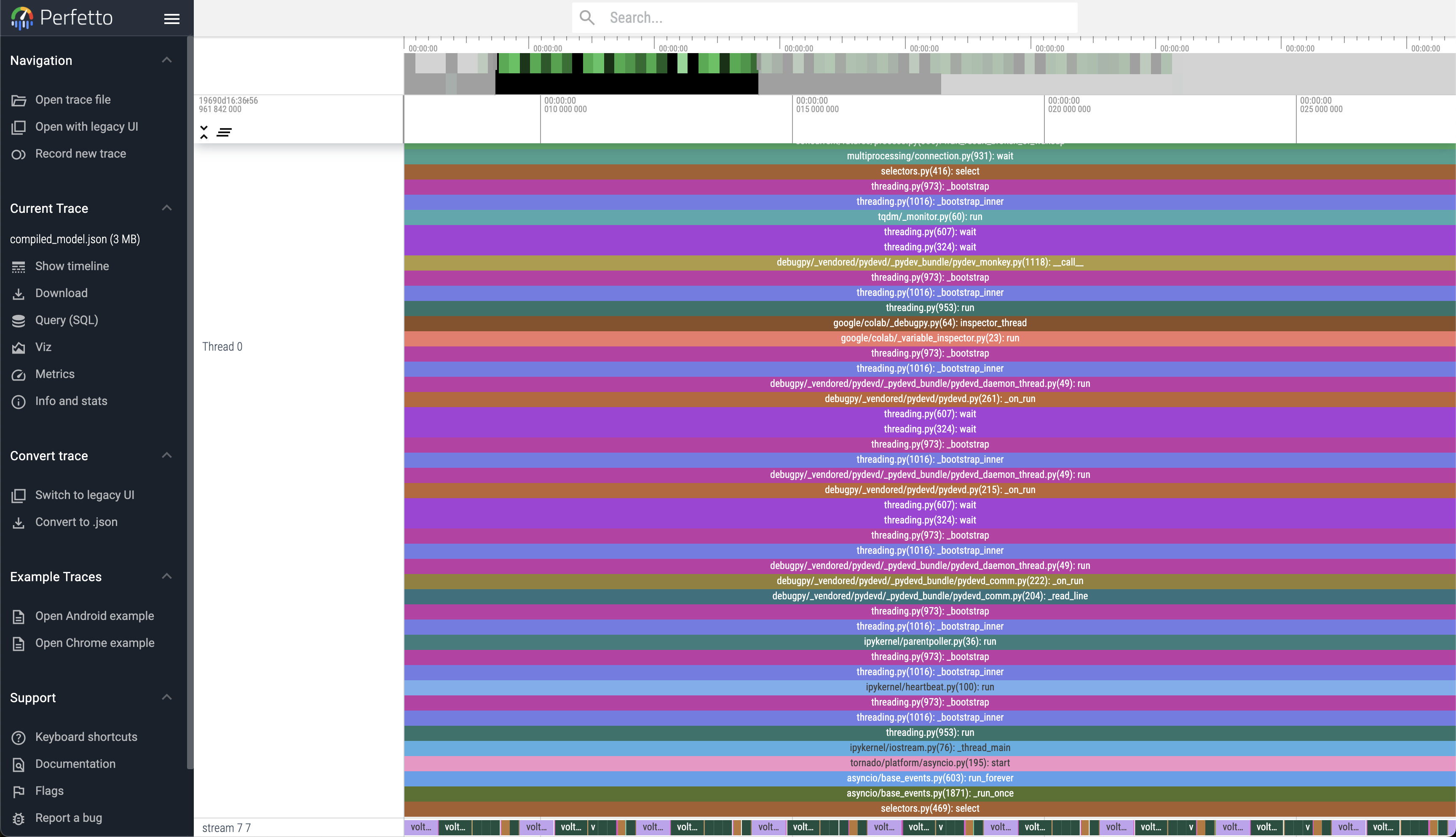
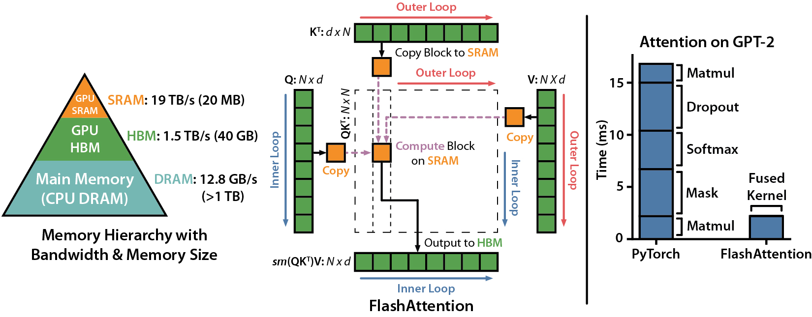
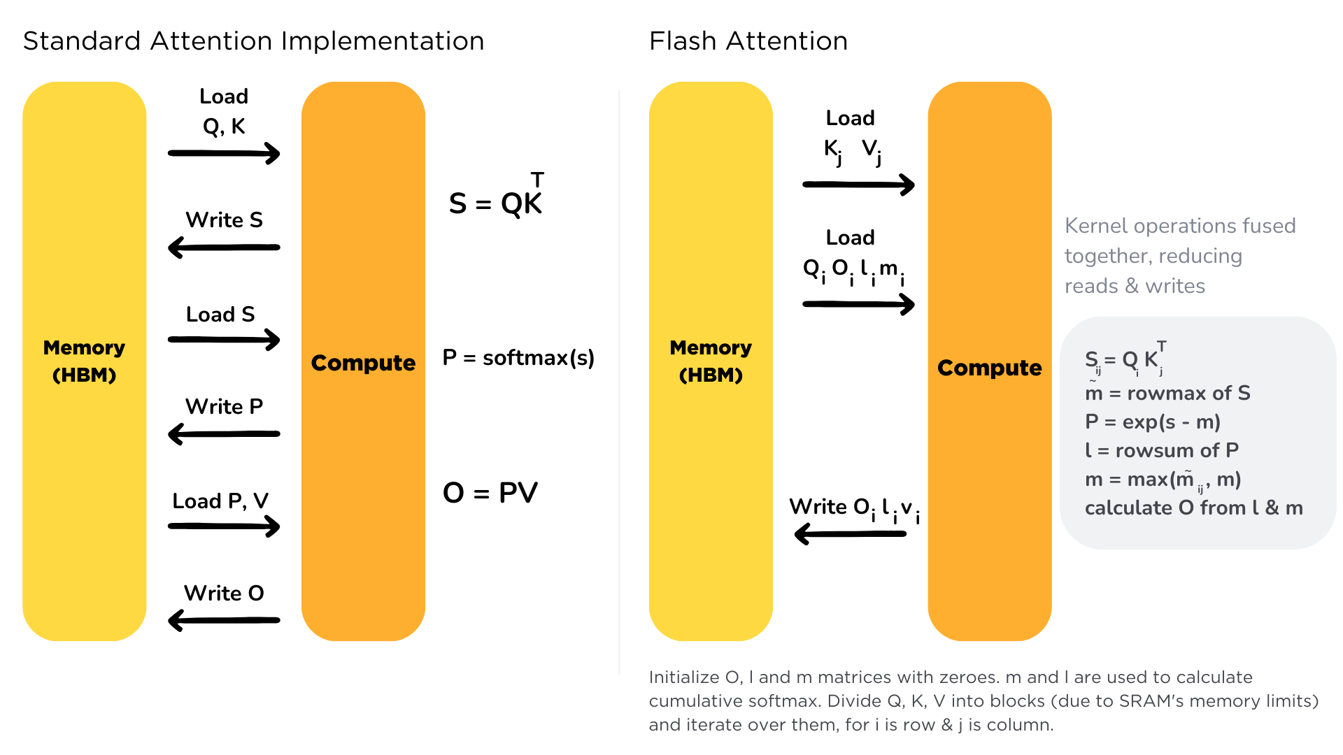
Flash Attention

FlashAttention-2 is a faster and more efficient implementation of the standard attention mechanism that can significantly speedup inference by:
- additionally parallelizing the attention computation over sequence length
- partitioning the work between GPU threads to reduce communication and shared memory reads/writes between them
FlashAttention-2 supports inference with Llama, Mistral, and Falcon models.
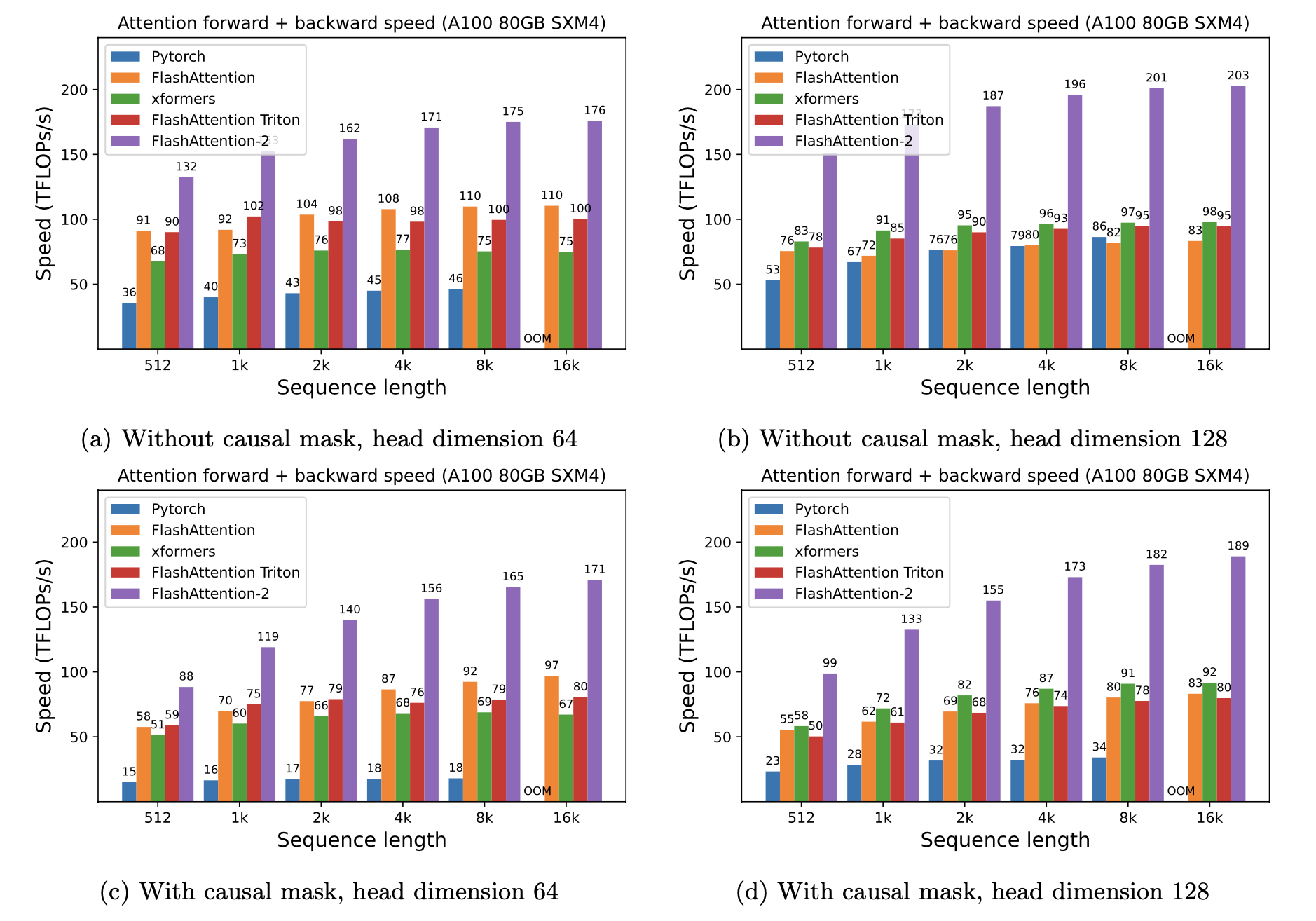
FlashAttention-2 currently supports:
- Ampere, Ada, or Hopper GPUs (e.g., A100, RTX 3090, RTX 4090, H100). Support for Turing GPUs (T4, RTX 2080) is coming soon, please use FlashAttention 1.x for Turing GPUs for now.
- Datatype fp16 and bf16 (bf16 requires Ampere, Ada, or Hopper GPUs).
- All head dimensions up to 256. Head dim > 192 backward requires A100/A800 or H100/H800.
Make sure to install the latest flash attention
pip install -U flash-attnOr install one from https://github.com/Dao-AILab/flash-attention/releases/tag/v2.3.6
Usage with transformers
import torch
from transformers import AutoModelForCausalLM, AutoTokenizer

checkpoint = "mistralai/Mistral-7B-v0.1"
device = "cuda" # for GPU usage or "cpu" for CPU usage

tokenizer = AutoTokenizer.from_pretrained(checkpoint)
model = AutoModelForCausalLM.from_pretrained(checkpoint, torch_dtype=torch.float16, use_flash_attention_2=True, low_cpu_mem_usage=True).to(device)

inputs = tokenizer.encode("Hello how are you?", return_tensors="pt").to(device)
outputs = model.generate(inputs, max_new_tokens=4, do_sample=False)
print(tokenizer.decode(outputs[0]))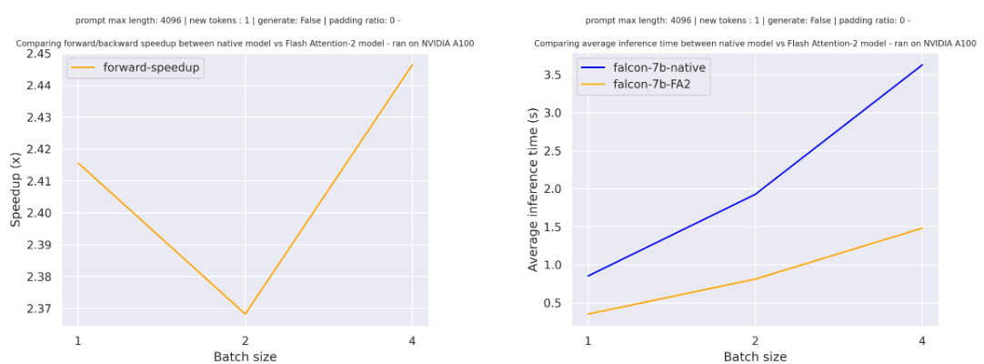
Scaled Dot Product Attention (PyTorch)
https://pytorch.org/docs/stable/generated/torch.nn.functional.scaled_dot_product_attention.html
PyTorch's Flash attention 2 (torch==2.2.0.dev20230915+cu121) runs at 490 ms/iter
Tri Dao's Flash attention 2 (flash-attn==2.2.2) runs at 483 ms/iter
GPU: NVIDIA A100-SXM4-40GB
Nvidia driver version: 525.105.17
from optimum.bettertransformer import BetterTransformer

bt_model = BetterTransformer.transform(model, keep_original_model=True)
OR
model.to_bettertransformer()This will use the fused kernel by default
It can be forced as well with with torch.backends.cuda.sdp_kernel(enable_math=False):
# Optionally use the context manager to ensure one of the fused kernels is run
query = torch.rand(32, 8, 128, 64, dtype=torch.float16, device="cuda")
key = torch.rand(32, 8, 128, 64, dtype=torch.float16, device="cuda")
value = torch.rand(32, 8, 128, 64, dtype=torch.float16, device="cuda")
with torch.backends.cuda.sdp_kernel(enable_math=False):
    F.scaled_dot_product_attention(query,key,value)
Colab Notebook:
https://colab.research.google.com/drive/1AD4rdEp1FxF6gmcVnHvp_nB1A55I0YWu?usp=sharing
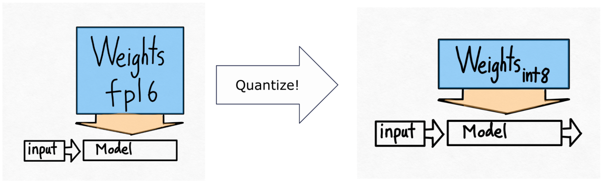
BitsAndBytes
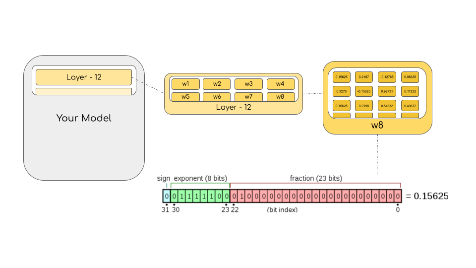
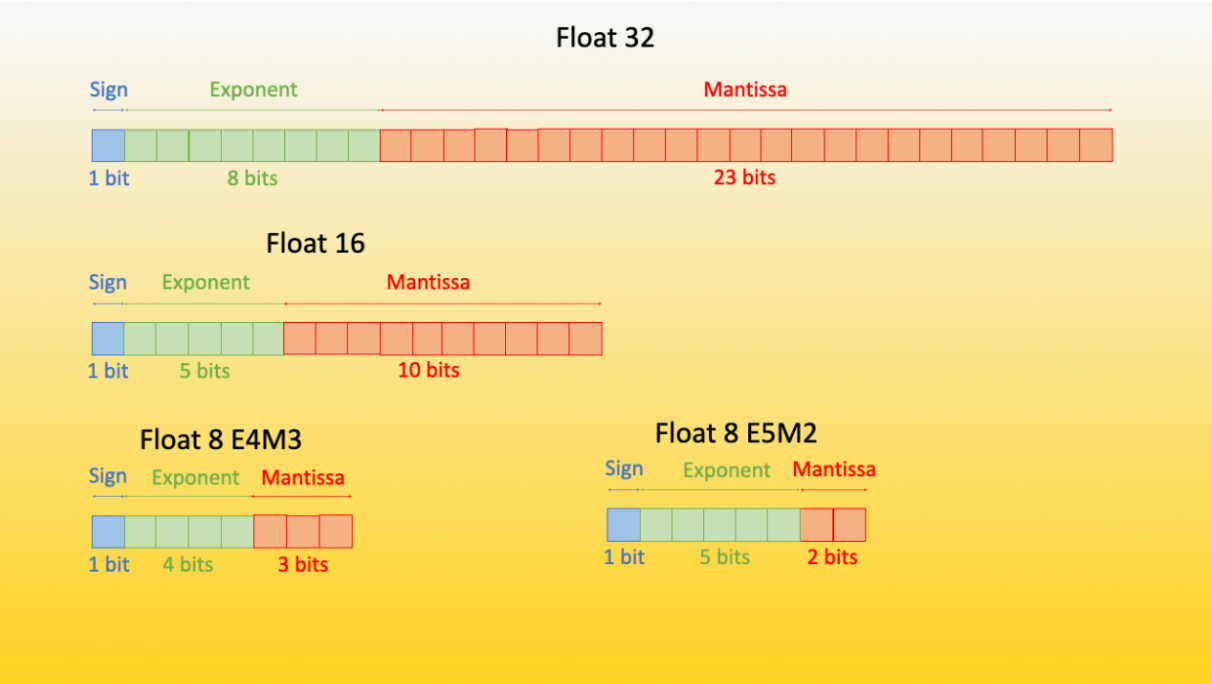
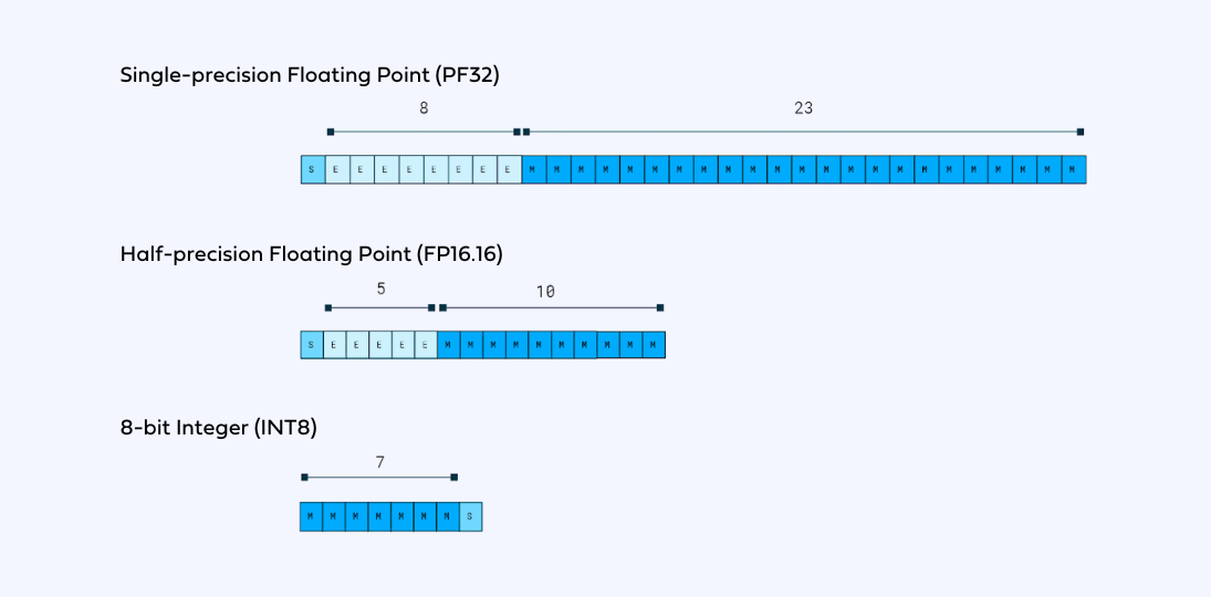
In the machine learning jargon FP32 is called full precision (4 bytes), while BF16 and FP16 are referred to as half-precision (2 bytes). On top of that, the int8 (INT8) data type consists of an 8-bit representation that can store 2^8 different values (between [0, 255] or [-128, 127] for signed integers).
https://github.com/TimDettmers/bitsandbytes
Source Code in Transformers
https://github.com/huggingface/transformers/blob/main/src/transformers/utils/quantization_config.py
Colab Notebook: https://colab.research.google.com/drive/1AD4rdEp1FxF6gmcVnHvp_nB1A55I0YWu?usp=sharing
FP16
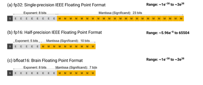
- FP32 (Float32): This is the standard IEEE 32-bit floating point representation. It has 23 bits for the mantissa, 8 bits for the exponent, and 1 sign bit. FP32 offers a wide range of representable values with good precision, making it the default choice for many computations. However, it requires more memory and computational resources compared to lower-precision formats.
- FP16 (Float16): FP16 cuts the number of bits in half compared to FP32, with 10 bits for the mantissa, 5 bits for the exponent, and 1 for the sign. The trade-off is a much smaller range of representable numbers and reduced precision. FP16 can cause numerical issues like overflow and underflow, where very large or small numbers respectively can't be accurately represented and lead to errors such as NaN (Not a Number).
- BF16 (BFloat16): To address the limitations of FP16 while not compromising too much on range, BF16 uses 8 bits for the exponent (like FP32) but only 7 bits for the mantissa. This keeps a wide dynamic range similar to FP32 but with slightly lower precision. BF16 strikes a balance that is suitable for many deep learning tasks where the wide range is more important than extreme precision.
- TF32 (TensorFloat-32): Exclusive to NVIDIA's Ampere architecture, TF32 offers a new format with 19 bits: 8 for the mantissa and 10 for the exponent. TF32 aims to balance range and precision by using more exponent bits than BF16 and fewer mantissa bits than FP32. It's used internally during specific GPU operations and offers the performance of FP16 with the range close to FP32.
Here we are trying to load a 1.7B model in FLOAT16
model = AutoModelForCausalLM.from_pretrained(
    "bigscience/bloom-1b7",
    device_map="auto",
    torch_dtype=torch.bfloat16,
)
tokenizer = AutoTokenizer.from_pretrained("bigscience/bloom-1b7")
INT8
Paper: https://arxiv.org/abs/2208.07339
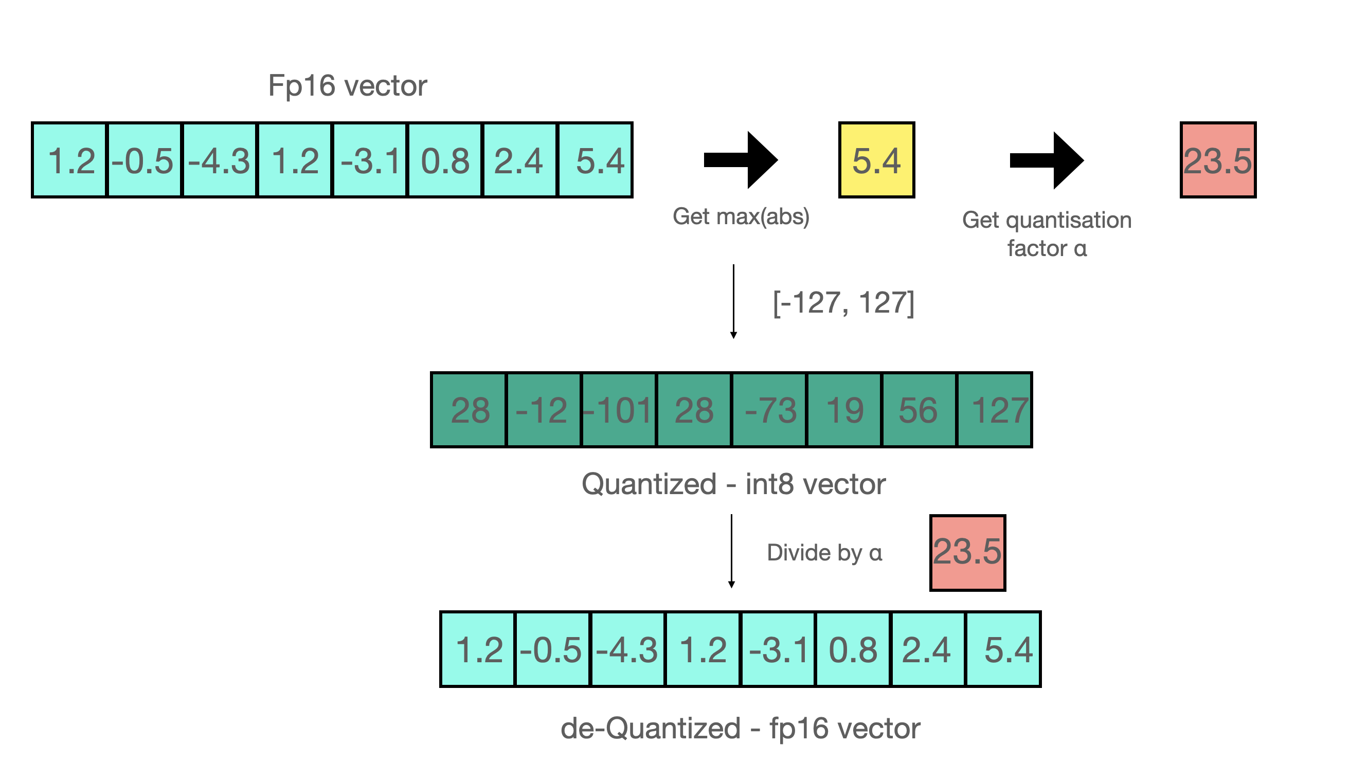
Absmax quantization is one type of quantization that scales numerical values to fit within the range of a target data type, such as int8.
Example of Absmax Quantization:
Assume you have a vector: [1.2, -0.5, -4.3, 1.2, -3.1, 0.8, 2.4, 5.4]. Here's how you perform absmax quantization:
- Find the absolute maximum number in the vector, which is
5.4. - Determine the range of the target quantization format, for int8 this is
[-127, 127]. - Calculate the scaling factor by dividing the maximum possible int8 value (
127) by the absolute maximum number (5.4), getting approximately23.5. - Quantize each number in the original vector by multiplying it by the scaling factor, giving you the quantized vector:
[28, -12, -101, 28, -73, 19, 56, 127].
LLM.int8(): zero degradation matrix multiplication for Large Language Models
The LLM.int8() method is designed for large language models (LLMs) to enable efficient inference (making predictions) with less computational resources without significant degradation in performance.
The operations of the LLM.int8() method are as follows:
- Outlier Extraction: Identify and extract outliers (elements exceeding a certain threshold) from the input data.
- Mixed-Precision Matrix Multiplication: Perform matrix multiplication where the outliers are processed using FP16 (for accuracy) and the non-outliers using int8 (for efficiency).
- Combination: Dequantize the results from the int8 computations back to FP16 and add them to the outlier computations, thus producing the final result.
The rationale behind LLM.int8() is to store data in int8 to save memory space while performing computations in FP16 to maintain the accuracy of the results. BLOOM-176B, a large language model, when using LLM.int8(), was found to be only slightly slower (about 15% to 23%) than its FP16 counterpart, which indicates that it is a viable solution for maintaining performance while being more resource-efficient.
This method is particularly useful when aiming to run large models on hardware with limited memory capacity or when trying to reduce costs associated with memory consumption and computation time. In your course, you can use this content to illustrate how numerical representation choices directly affect both the storage and computational aspects of model deployment
eight_bit_config = BitsAndBytesConfig(
    load_in_8bit=True
)

model = AutoModelForCausalLM.from_pretrained(
    "bigscience/bloom-1b7",
    device_map="auto",
    quantization_config=eight_bit_config
)
tokenizer = AutoTokenizer.from_pretrained("bigscience/bloom-1b7")
INT4
Quantization technique is same as INT8 but now instead you have -8 to 7 as the values
four_bit_config = BitsAndBytesConfig(
    load_in_4bit=True
)

model = AutoModelForCausalLM.from_pretrained(
    "bigscience/bloom-1b7",
    device_map="auto",
    quantization_config=four_bit_config
)
tokenizer = AutoTokenizer.from_pretrained("bigscience/bloom-1b7")
NF4
Consider a weight in the neural network that is represented by a 32-bit floating-point number, with the value 0.5678.
Now, we want to quantize this weight to a 4-bit integer. In our example, a 4-bit integer can represent 16 evenly spaced levels between -1 and 1. The levels are:
-1.0, -0.8667, -0.7333, -0.6, -0.4667, -0.3333, -0.2, -0.0667,
0.0667, 0.2, 0.3333, 0.4667, 0.6, 0.7333, 0.8667, 1.0
To quantize the weight 0.5678, we find the nearest level in our 4-bit representation, which is 0.6.
Let's say that the level 0.6 is associated with the 4-bit integer value 13. We would then store the integer 13 instead of the original 32-bit floating-point number (0.5678).
In a computation, whenever this weight is needed, we dequantize the 4-bit integer back to the original level 0.6 before using it in calculations. This means we are introducing a quantization error, which is the difference between the dequantized value and the original floating-point value:
Dequantization error = Dequantized value - Original value
                     = 0.6 - 0.5678
                     = 0.0322
In this example, the error is 0.0322. This is approximately one-fourth of the distance between two quantization levels (since 1 / (1/0.1333) = 1 / 7.5 ≈ 0.1333, and 0.1333 / 4 ≈ 0.0333).
For enabling nested quantization, you can use the bnb_4bit_use_double_quant argument in BitsAndBytesConfig. This will enable a second quantization after the first one to save an additional 0.4 bits per parameter.
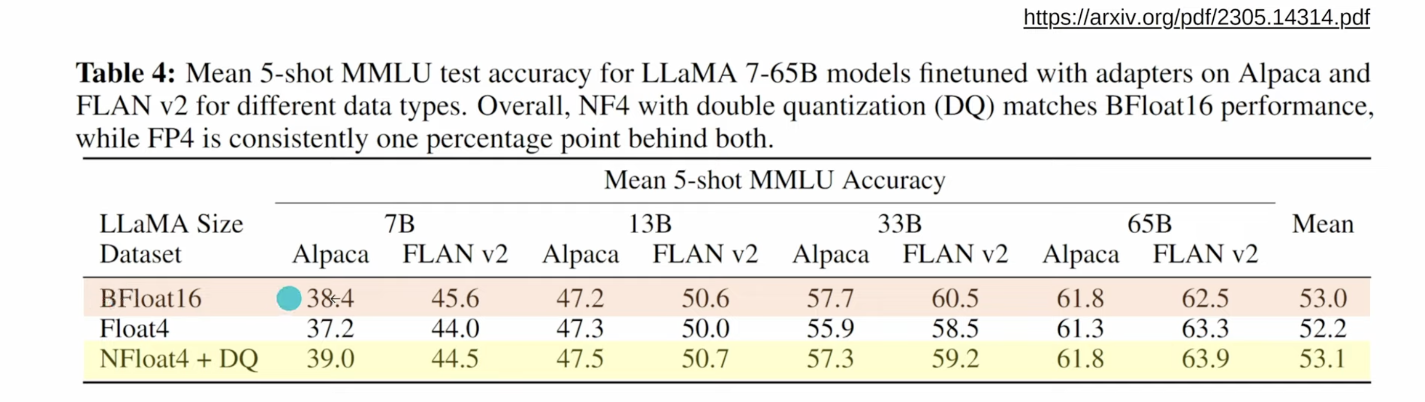
- Both NF4 and FP4 show comparable performance in terms of inference speed, memory consumption, and the quality of content generation.
- NF4 demonstrates better stability at lower temperatures with the LLaMA2 series of models. This stability is crucial for maintaining model performance in changing thermal environments.
- FP4, and its variant FP4-DQ (where DQ stands for Double Quantization), is found to be more appropriate for the Falcon series of models.
- Generally, 4-bit quantized models are more sensitive to temperature variations compared to unquantized models, with greater sensitivity noted in the temperature range of 0.5 to 0.8.
Premise of NF4:
- NF4 is designed to optimize quantization for neural network weights that typically exhibit a zero-centered normal distribution, eliminating the need for expensive quantile estimates.
- This approach is feasible because input tensors can be transformed to adhere to a fixed distribution up to a quantization constant.
- The method's validity is supported by the Shapiro-Wilk test, indicating that the vast majority (approximately 92.5%) of the LLaMA neural network weights follow a normal distribution.
Key Concepts Explained:
- NF4 (4-bit NormalFloat):
- An optimal quantization data type specifically for data that follows a normal distribution.
- It uses Quantile Quantization and is estimated using a quantile approximation algorithm based on the zero-mean normal distribution of pre-trained neural network weights.
- Double Quantization (DQ):
- A method that further quantizes the quantization constants (used for initial quantization) into a lower-precision format, resulting in memory savings.
- For example, saving approximately 3 GB of memory for a 65 billion parameter model.
- FP4-DQ involves applying FP4 quantization to the initial quantization constants, reducing these constants to 8-bit precision (FP8).
Additional Context for NF4:
- NF4 aims to create a quantization scheme that's tailored to the characteristics of neural networks, where weights and activations often assume a distribution close to the normal distribution.
- The adoption of NF4 and FP4-DQ is part of efforts like QLoRA to optimize the fine-tuning of quantized large language models (LLMs), maintaining efficiency while keeping computational overhead low.
nf4_config = BitsAndBytesConfig(
    load_in_4bit=True,
    bnb_4bit_quant_type="nf4",
    bnb_4bit_use_double_quant=True,
    bnb_4bit_compute_dtype=torch.bfloat16
)

model = AutoModelForCausalLM.from_pretrained(
    "bigscience/bloom-1b7",
    device_map="auto",
    quantization_config=nf4_config
)
tokenizer = AutoTokenizer.from_pretrained("bigscience/bloom-1b7")
INT8/INT4 with Flash Attention 2
FlashAttention-2 can be combined with other optimization techniques like quantization to further speedup inference. For example, you can combine FlashAttention-2 with 8-bit or 4-bit quantization:
import torch
from transformers import AutoModelForCausalLM, AutoTokenizer, LlamaForCausalLM

model_id = "tiiuae/falcon-7b"
tokenizer = AutoTokenizer.from_pretrained(model_id)

# load in 8bit
model = AutoModelForCausalLM.from_pretrained(
    model_id,
    load_in_8bit=True,
    use_flash_attention_2=True,
)

# load in 4bit
model = AutoModelForCausalLM.from_pretrained(
    model_id,
    load_in_4bit=True,
    use_flash_attention_2=True,
)
CPU Offloading
https://huggingface.co/docs/accelerate/usage_guides/quantization CPU and Disk Offloading
https://huggingface.co/docs/transformers/main_classes/quantization#offload-between-cpu-and-gpu
Offload between cpu and gpu
One of the advanced use case of this is being able to load a model and dispatch the weights between CPU and GPU. Note that the weights that will be dispatched on CPU will not be converted in 8-bit, thus kept in float32. This feature is intended for users that want to fit a very large model and dispatch the model between GPU and CPU.
device_map = {
    "transformer.word_embeddings": 0,
    "transformer.word_embeddings_layernorm": 0,
    "lm_head": "cpu",
    "transformer.h": 0,
    "transformer.ln_f": 0,
}
model = AutoModelForCausalLM.from_pretrained(
"bigscience/bloom-1b7",
device_map=device_map,
quantization_config=quantization_config,
)AWQ
AWQ method has been introduced in the *AWQ: Activation-aware Weight Quantization for LLM Compression and Acceleration* paper. With AWQ you can run models in 4-bit precision, while preserving its original quality (i.e. no performance degradation) with a superior throughput that other quantization methods presented below - reaching similar throughput as pure float16 inference.
Hands-On
https://colab.research.google.com/drive/1ppBB9f1l7NBEuvjs3BTwn43Kry8rneB4?usp=sharing
quant_config = {"zero_point": True, "q_group_size": 128, "w_bit": 4, "version":"GEMM"}

model = AutoAWQForCausalLM.from_pretrained("facebook/opt-1.3b")
tokenizer = AutoTokenizer.from_pretrained("facebook/opt-1.3b", trust_remote_code=True)
from transformers import AwqConfig, AutoConfig
# modify the config file so that it is compatible with transformers integration
quantization_config = AwqConfig(
bits=quant_config["w_bit"],
group_size=quant_config["q_group_size"],
zero_point=quant_config["zero_point"],
version=quant_config["version"].lower(),
).to_dict()
# the pretrained transformers model is stored in the model attribute + we need to pass a dict
model.model.config.quantization_config = quantization_config
# a second solution would be to use Autoconfig and push to hub (what we do at llm-awq)
# save model weights
model.save_quantized("opt-1.3b-awq")
tokenizer.save_pretrained("opt-1.3b-awq")GPTQ
https://github.com/PanQiWei/AutoGPTQ
Original Paper Code: https://github.com/IST-DASLab/gptq
Paper: https://arxiv.org/abs/2210.17323
GPTQ adopts a mixed int4/fp16 quantization scheme where weights are quantized as int4 while activations remain in float16. During inference, weights are dequantized on the fly and the actual compute is performed in float16.
The benefits of this scheme are twofold:
- Memory savings close to x4 for int4 quantization, as the dequantization happens close to the compute unit in a fused kernel, and not in the GPU global memory.
- Potential speedups thanks to the time saved on data communication due to the lower bitwidth used for weights.
GPTQ uses a Cholesky decomposition, a numerically stable method for solving certain mathematical problems. It involves precomputing some required information from the matrix using the Cholesky method. This approach, combined with a slight “dampening” (adding a small constant to diagonal elements of the matrix), helps the algorithm to avoid numerical issues.
The full algorithm can be summarized in a few steps:
- The GPTQ algorithm begins with a Cholesky decomposition of the Hessian inverse (a matrix that helps decide how to adjust the weights)
- It then runs in loops, handling batches of columns at a time.
- For each column in a batch, it quantizes the weights, calculates the error, and updates the weights in the block accordingly.
- After processing the batch, it updates all remaining weights based on the block’s errors.
Basically it will try to quantize the entire column in the weight matrix, if it finds that it creates a lot of error in the model output (deviations pre quantization) then that column is not quantized, if it’s within threshold it quantizes it.
Reference: https://mlabonne.github.io/blog/posts/4_bit_Quantization_with_GPTQ.html
This supports 2,3,4 bits quantizations
Hands-On
https://colab.research.google.com/drive/153rJG9dVDk8OnvWRX6gQBtnHkRYjY3-w?usp=sharing
quantization_config = GPTQConfig(
     bits=4,
     group_size=128,
     dataset="c4",
     desc_act=False,
)
But what’s this group size?
When we put a neural network "parameter" from 32-bit or 16-bit floating numbers, all the way down to int4, or int3, there is a need for a scaling factor which would translate 16 combinations of int4, or 8 combinations of int3, into an essentially unlimited range of floating point numbers.
We need "scaling weights" which allows us to translate these integers into a large variety of values.
This is done by assigning "scaling weights" to a collection of neural network "parameters", let's just say one exponential and another linear (so that we can obtain a zero, somehow). The natural way of thinking is that we assign it to a full "row" (let's say, for example, 4096 of them) of these "parameters".
The groupsize 128 (or 32, for the matter), is making it such the scaling parameters are shared by not all members of a row, but just 32, or 128 of those "parameters".
The effect of having less parameters sharing a scaling function is that the scaling become more accurate and efficient.
tokenizer = AutoTokenizer.from_pretrained("facebook/opt-1.3b")
quant_model = AutoModelForCausalLM.from_pretrained("facebook/opt-1.3b", quantization_config=quantization_config, device_map='auto')
you can use model.config.model_type to compare with the table below to check whether the model you use is supported by auto_gptq.
for example, model_type of WizardLM, vicuna and gpt4all are all llama, hence they are all supported by auto_gptq.
For quantizing a model using auto-gptq, we need to pass a dataset to the quantizer. This can be achieved either by passing a supported default dataset among ['wikitext2','c4','c4-new','ptb','ptb-new'] or a list of strings that will be used as a dataset.
| model type | quantization | inference | peft-lora | peft-ada-lora | peft-adaption_prompt |
|---|---|---|---|---|---|
| bloom | ✅ | ✅ | ✅ | ✅ | |
| gpt2 | ✅ | ✅ | ✅ | ✅ | |
| gpt_neox | ✅ | ✅ | ✅ | ✅ | ✅https://github.com/PanQiWei/peft/tree/multi_modal_adaption_prompt |
| gptj | ✅ | ✅ | ✅ | ✅ | ✅https://github.com/PanQiWei/peft/tree/multi_modal_adaption_prompt |
| llama | ✅ | ✅ | ✅ | ✅ | ✅ |
| moss | ✅ | ✅ | ✅ | ✅ | ✅https://github.com/PanQiWei/peft/tree/multi_modal_adaption_prompt |
| opt | ✅ | ✅ | ✅ | ✅ | |
| gpt_bigcode | ✅ | ✅ | ✅ | ✅ | |
| codegen | ✅ | ✅ | ✅ | ✅ | |
| falcon(RefinedWebModel/RefinedWeb) | ✅ | ✅ | ✅ | ✅ |
PEFT (Parameter Efficient FineTuning)
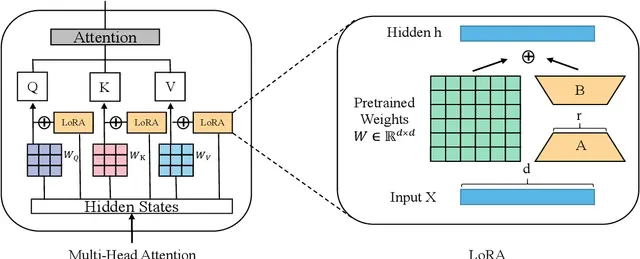
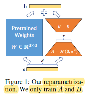
- LoRA: LORA: LOW-RANK ADAPTATION OF LARGE LANGUAGE MODELS
- Prefix Tuning: Prefix-Tuning: Optimizing Continuous Prompts for Generation, P-Tuning v2: Prompt Tuning Can Be Comparable to Fine-tuning Universally Across Scales and Tasks
- P-Tuning: GPT Understands, Too
- Prompt Tuning: The Power of Scale for Parameter-Efficient Prompt Tuning
- AdaLoRA: Adaptive Budget Allocation for Parameter-Efficient Fine-Tuning
- (��)3: Few-Shot Parameter-Efficient Fine-Tuning is Better and Cheaper than In-Context Learning
- MultiTask Prompt Tuning: Multitask Prompt Tuning Enables Parameter-Efficient Transfer Learning
- LoHa: FedPara: Low-Rank Hadamard Product for Communication-Efficient Federated Learning
- LoKr: KronA: Parameter Efficient Tuning with Kronecker Adapter based on Navigating Text-To-Image Customization:From LyCORIS Fine-Tuning to Model Evaluation implementation
- LoftQ: LoftQ: LoRA-Fine-Tuning-aware Quantization for Large Language Models
- OFT: Controlling Text-to-Image Diffusion by Orthogonal Finetuning
Hardware: Single A100 80GB GPU with CPU RAM above 64GB
| Model | Full Finetuning | PEFT-LoRA PyTorch | PEFT-LoRA DeepSpeed with CPU Offloading |
|---|---|---|---|
| bigscience/T0_3B (3B params) | 47.14GB GPU / 2.96GB CPU | 14.4GB GPU / 2.96GB CPU | 9.8GB GPU / 17.8GB CPU |
| bigscience/mt0-xxl (12B params) | OOM GPU | 56GB GPU / 3GB CPU | 22GB GPU / 52GB CPU |
| bigscience/bloomz-7b1 (7B params) | OOM GPU | 32GB GPU / 3.8GB CPU | 18.1GB GPU / 35GB CPU |
LORA (Low Rank Adaptation)
DeepSpeed
https://huggingface.co/docs/transformers/main_classes/deepspeed
DeepSpeed implements everything described in the ZeRO paper (Zero Redundancy Optimizer). Currently it provides full support for:
- Optimizer state partitioning (ZeRO stage 1)
- Gradient partitioning (ZeRO stage 2)
- Parameter partitioning (ZeRO stage 3)
- Custom mixed precision training handling
- A range of fast CUDA-extension-based optimizers
- ZeRO-Offload to CPU and NVMe
The Zero Redundancy Optimizer (ZeRO) removes the memory redundancies across data-parallel processes by partitioning the three model states (optimizer states, gradients, and parameters) across data-parallel processes instead of replicating them. By doing this, it boosts memory efficiency compared to classic data-parallelism while retaining its computational granularity and communication efficiency.
- ZeRO Stage 1: The optimizer states (e.g., for Adam optimizer, 32-bit weights, and the first, and second moment estimates) are partitioned across the processes, so that each process updates only its partition.
- ZeRO Stage 2: The reduced 32-bit gradients for updating the model weights are also partitioned such that each process retains only the gradients corresponding to its portion of the optimizer states.
- ZeRO Stage 3: The 16-bit model parameters are partitioned across the processes. ZeRO-3 will automatically collect and partition them during the forward and backward passes.
With PyTorch Lightning
Lightning Fabric
Fabric is the fast and lightweight way to scale PyTorch models without boilerplate. Convert PyTorch code to Lightning Fabric in 5 lines and get access to SOTA distributed training features (DDP, FSDP, DeepSpeed, mixed precision and more) to scale the largest billion-parameter models.
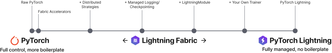
Fabric differentiates itself from a fully-fledged trainer like Lightning’s Trainer in these key aspects:
Fast to implement There is no need to restructure your code: Just change a few lines in the PyTorch script and you’ll be able to leverage Fabric features.
Maximum Flexibility Write your own training and/or inference logic down to the individual optimizer calls. You aren’t forced to conform to a standardized epoch-based training loop like the one in Lightning Trainer. You can do flexible iteration based training, meta-learning, cross-validation and other types of optimization algorithms without digging into framework internals. This also makes it super easy to adopt Fabric in existing PyTorch projects to speed-up and scale your models without the compromise on large refactors. Just remember: With great power comes a great responsibility.
Maximum Control The Lightning Trainer has many built-in features to make research simpler with less boilerplate, but debugging it requires some familiarity with the framework internals. In Fabric, everything is opt-in. Think of it as a toolbox: You take out the tools (Fabric functions) you need and leave the other ones behind. This makes it easier to develop and debug your PyTorch code as you gradually add more features to it. Fabric provides important tools to remove undesired boilerplate code (distributed, hardware, checkpoints, logging, …), but leaves the design and orchestration fully up to you.
BitsAndBytes: https://lightning.ai/blog/8-bit-quantization-with-lightning-fabric/
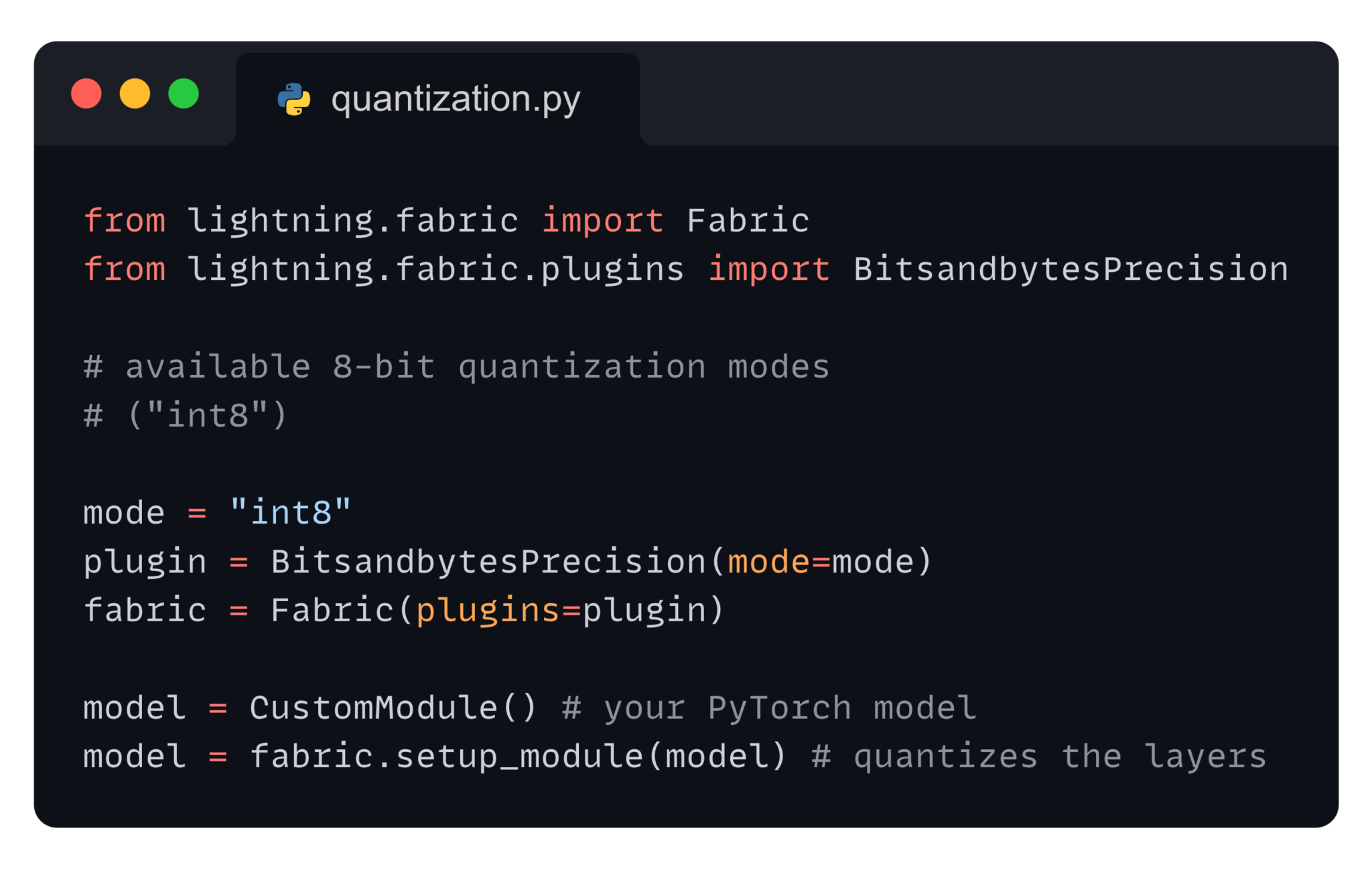
https://lightning.ai/docs/fabric/latest/fundamentals/precision.html#quantization-via-bitsandbytes
from lightning.fabric.plugins import BitsandbytesPrecision

# this will pick out the compute dtype automatically, by default `bfloat16`
precision = BitsandbytesPrecision(mode="nf4-dq")
fabric = Fabric(plugins=precision)

# Customize the dtype, or ignore some modules
precision = BitsandbytesPrecision(mode="int8-training", dtype=torch.float16, ignore_modules={"lm_head"})
fabric = Fabric(plugins=precision)

model = MyModel()
model = fabric.setup(model)
LLM Optimization with Pytorch 2.0
This came in 17 hours after i finished creating this content 😭
https://pytorch.org/blog/accelerating-generative-ai-2/
Make sure to install the latest nightly release of pytorch 2 !
pip3 install --pre torch torchvision torchaudio --index-url https://download.pytorch.org/whl/nightly/cu121>>> import torch
>>> torch.__version__
'2.2.0.dev20231201+cu121'
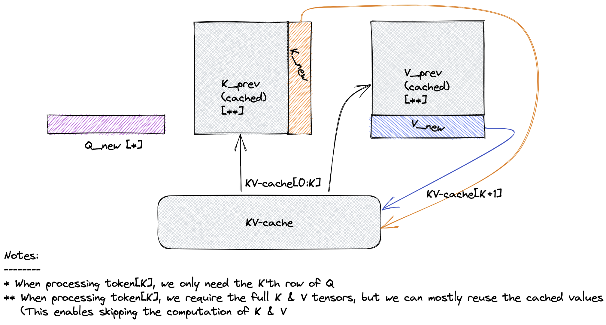
>>>Step 1: torch.compile and kv-cache
Step 2: INT8 Quantization
Step 3: Speculative Decoding
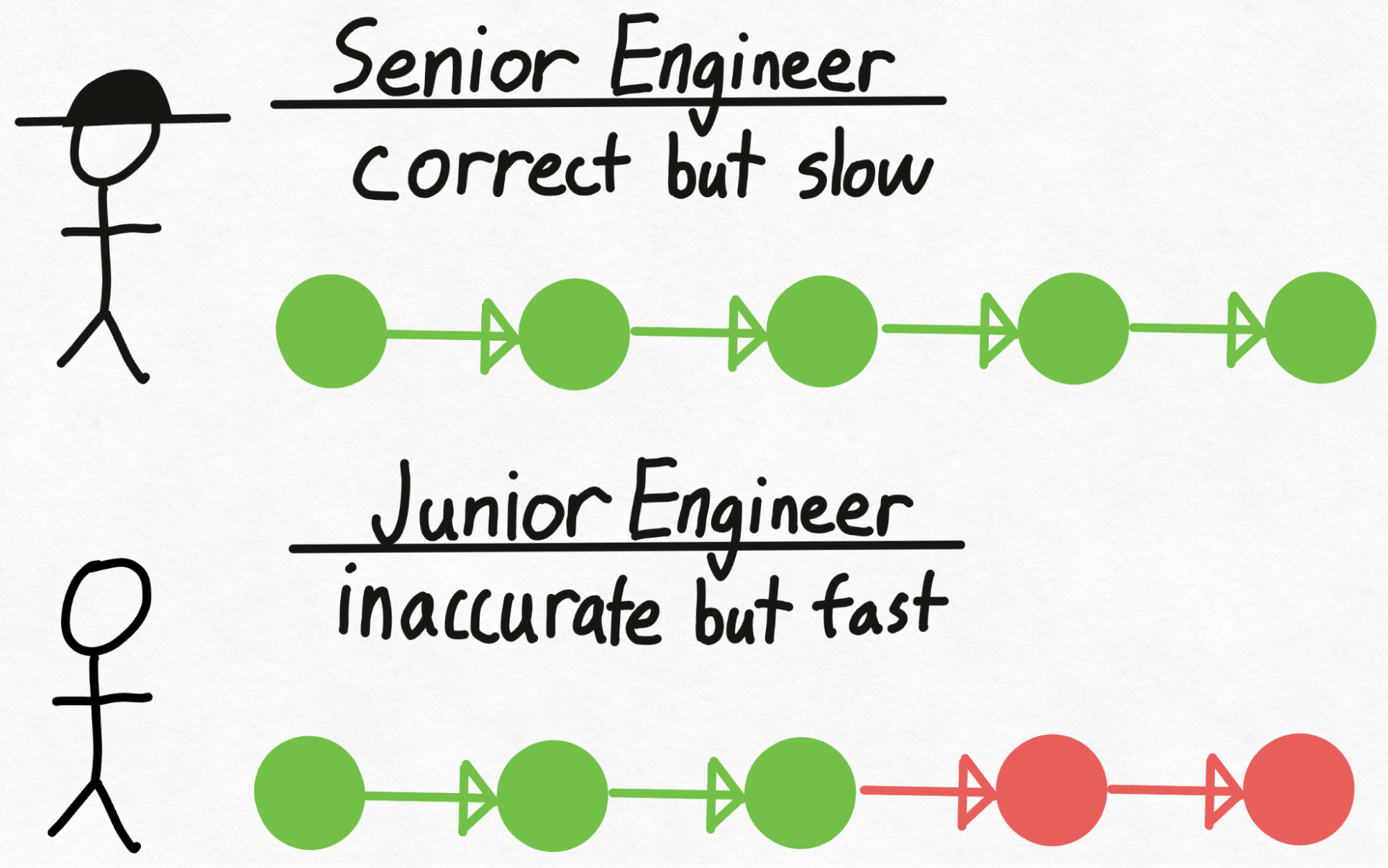
- Select a small model and a large one of your preference. Make sure they share the same tokenizer, so that we can meaningfully compare the logits of the two models.
- Generate a specific number of candidate new tokens with the small model, say 3. This involves running the forward pass on the small model 3 times.
- Use the larger model to forward pass the prospective new input (combining the original with the 3 new tokens). This returns lists of potential tokens with their corresponding probabilities for all input tokens.
- Decode the last 4 tokens using greedy decoding (3 new tokens plus an additional one from the forward pass of the large model). Compare the decoded tokens from the large model with the candidate new tokens, starting from left to right. If the tokens match, we accept them and append them to the original input. Continue this process until the first mismatch occurs, at which point we append the token from the large model to the input. This updated input is then passed through the small model to generate 3 more tokens, and the entire process is repeated.
Step 4: INT4 Quantization and GPTQ
Of course, if reducing the weights down from 16 bits to 8 bits allows for speedups by reducing the number of bytes we need to load, reducing the weights down to 4 bits would result in even larger speedups!
Unfortunately, when reducing weights down to 4-bits, the accuracy of the model starts to become a much larger concern. From our preliminary evals, we see that although using int8 weight-only quantization has no perceptible accuracy degradation, using int4 weight-only quantization does.
codellama/CodeLlama-7b-Python-hf
codellama/CodeLlama-34b-Python-hf
git clone https://github.com/pytorch-labs/gpt-fastexport MODEL_REPO=codellama/CodeLlama-7b-Python-hf
./scripts/prepare.sh $MODEL_REPO❯ export MODEL_REPO=codellama/CodeLlama-7b-Python-hf
./scripts/prepare.sh $MODEL_REPO
config.json: 100%|████████████████████████████████████████████████████████████████████████████████████████████████████████| 644/644 [00:00<00:00, 58.4kB/s]
README.md: 100%|███████████████████████████████████████████████████████████████████████████████████████████████████████| 6.17k/6.17k [00:00<00:00, 570kB/s]
LICENSE: 100%|████████████████████████████████████████████████████████████████████████████████████████████████████████| 7.02k/7.02k [00:00<00:00, 1.25MB/s]
generation_config.json: 100%|█████████████████████████████████████████████████████████████████████████████████████████████| 116/116 [00:00<00:00, 23.6kB/s]
USE_POLICY.md: 100%|███████████████████████████████████████████████████████████████████████████████████████████████████| 4.79k/4.79k [00:00<00:00, 772kB/s]
.gitattributes: 100%|██████████████████████████████████████████████████████████████████████████████████████████████████| 1.52k/1.52k [00:00<00:00, 279kB/s]
model.safetensors.index.json: 100%|███████████████████████████████████████████████████████████████████████████████████| 25.1k/25.1k [00:00<00:00, 2.72MB/s]
special_tokens_map.json: 100%|█████████████████████████████████████████████████████████████████████████████████████████████| 411/411 [00:00<00:00, 276kB/s]
pytorch_model.bin.index.json: 100%|███████████████████████████████████████████████████████████████████████████████████| 23.9k/23.9k [00:00<00:00, 18.8MB/s]
tokenizer_config.json: 100%|███████████████████████████████████████████████████████████████████████████████████████████████| 749/749 [00:00<00:00, 494kB/s]
tokenizer.json: 100%|█████████████████████████████████████████████████████████████████████████████████████████████████| 1.84M/1.84M [00:01<00:00, 1.62MB/s]
tokenizer.model: 100%|██████████████████████████████████████████████████████████████████████████████████████████████████| 500k/500k [00:00<00:00, 1.63MB/s]
model-00002-of-00002.safetensors: 100%|███████████████████████████████████████████████████████████████████████████████| 3.50G/3.50G [02:41<00:00, 21.6MB/s]
pytorch_model-00003-of-00003.bin: 100%|███████████████████████████████████████████████████████████████████████████████| 3.59G/3.59G [02:56<00:00, 20.3MB/s]
pytorch_model-00002-of-00003.bin: 100%|███████████████████████████████████████████████████████████████████████████████| 4.95G/4.95G [03:28<00:00, 23.8MB/s]
pytorch_model-00001-of-00003.bin: 100%|███████████████████████████████████████████████████████████████████████████████| 4.94G/4.94G [03:37<00:00, 22.7MB/s]
model-00001-of-00002.safetensors: 100%|███████████████████████████████████████████████████████████████████████████████| 9.98G/9.98G [05:04<00:00, 32.8MB/s]
Fetching 17 files: 100%|███████████████████████████████████████████████████████████████████████████████████████████████████| 17/17 [05:09<00:00, 18.18s/it]
Model config {'block_size': 16384, 'vocab_size': 32000, 'n_layer': 32, 'n_head': 32, 'dim': 4096, 'intermediate_size': 11008, 'n_local_heads': 32, 'head_dim': 128, 'rope_base': 1000000, 'norm_eps': 1e-05}█████████████████████████████████████████████████████████████████████| 4.95G/4.95G [03:28<00:00, 33.5MB/s]
Saving checkpoint to checkpoints/codellama/CodeLlama-7b-Python-hf/model.pth
Loading model ...
Quantizing model weights for int8 weight-only symmetric per-channel quantization
Writing quantized weights to checkpoints/codellama/CodeLlama-7b-Python-hf/model_int8.pth
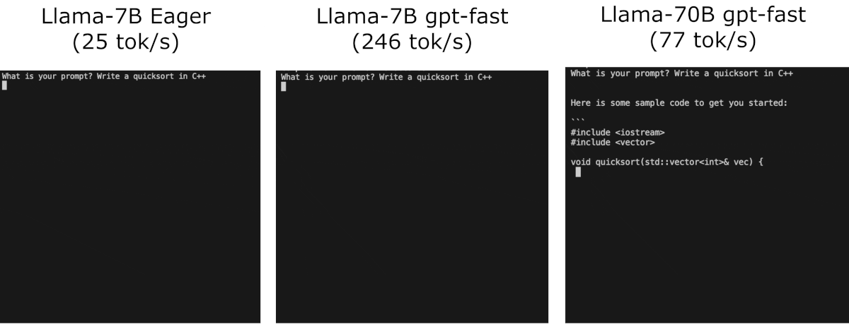
Quantization complete took 30.24 secondsVanilla (No Optimizations)
Disable KV Cache by commenting out this: https://github.com/pytorch-labs/gpt-fast/blob/3bcaaaf068d112d534f335ec21a17d7b8b5551bf/generate.py#L154
python generate.py --checkpoint_path checkpoints/$MODEL_REPO/model.pth --prompt "def quick_sort("Time for inference 1: 9.88 sec total, 20.24 tokens/sec
Bandwidth achieved: 272.71 GB/sTorch Compile
python generate.py --compile --checkpoint_path checkpoints/$MODEL_REPO/model.pth --prompt "def quick_sort("KV Caching is by default enabled!
https://github.com/pytorch-labs/gpt-fast/blob/3bcaaaf068d112d534f335ec21a17d7b8b5551bf/model.py#L94
def setup_caches(self, max_batch_size, max_seq_length):
        if self.max_seq_length >= max_seq_length and self.max_batch_size >= max_batch_size:
            return
        head_dim = self.config.dim // self.config.n_head
        max_seq_length = find_multiple(max_seq_length, 8)
        self.max_seq_length = max_seq_length
        self.max_batch_size = max_batch_size
        for b in self.layers:
            b.attention.kv_cache = KVCache(max_batch_size, max_seq_length, self.config.n_local_heads, head_dim)

        self.freqs_cis = precompute_freqs_cis(self.config.block_size, self.config.dim // self.config.n_head, self.config.rope_base)
        self.causal_mask = torch.tril(torch.ones(self.max_seq_length, self.max_seq_length, dtype=torch.bool))
Time for inference 5: 3.18 sec total, 62.88 tokens/sec
Bandwidth achieved: 847.45 GB/s
==========
Average tokens/sec: 62.90
Memory used: 13.92 GBWith INT8
python generate.py --compile --checkpoint_path checkpoints/$MODEL_REPO/model_int8.pth --prompt "def quick_sort("Time for inference 5: 1.92 sec total, 104.43 tokens/sec
Bandwidth achieved: 717.67 GB/s
==========
Average tokens/sec: 104.57
Memory used: 7.78 GBWith INT4
python quantize.py --checkpoint_path checkpoints/$MODEL_REPO/model.pth --mode int4 --groupsize 32python generate.py --checkpoint_path checkpoints/$MODEL_REPO/model_int4.g32.pth --compile --prompt "def quick_sort("Time for inference 5: 1.23 sec total, 162.60 tokens/sec
Bandwidth achieved: 714.17 GB/s
==========
Average tokens/sec: 162.67
Memory used: 4.92 GBSpeculative Sampling
python generate.py --compile --checkpoint_path checkpoints/$MODEL_REPO/model.pth --draft_checkpoint_path checkpoints/$MODEL_REPO/model_int8.pth --prompt "def quick_sort("Here the draft model is simply the int8 version of the same model
Time for inference 5: 2.58 sec total, 77.57 tokens/sec
Bandwidth achieved: 1045.44 GB/s
==========
Acceptance probs: [0.014423076923076924, 0.014423076923076924, 0.009615384615384616, 0.009615384615384616, 0.009615384615384616, 0.9423076923076923]
Mean Accepted: 4.8125
Average tokens/sec: 76.72
Memory used: 21.37 GB
Here we have the full FP16 model but with INT8 as the draft model, the speed and quality is just ❤️

NOTES
- MMLU Benchmark: https://huggingface.co/blog/evaluating-mmlu-leaderboard
- All options for BitsAndBytes: https://colab.research.google.com/drive/1ge2F1QSK8Q7h0hn3YKuBCOAS0bK8E0wf
- BitsAndBytes in HF: https://huggingface.co/blog/hf-bitsandbytes-integration
- Optimizing SAM: https://pytorch.org/blog/accelerating-generative-ai/
- GPT KV Cache: https://www.dipkumar.dev/becoming-the-unbeatable/posts/gpt-kvcache/
- PyTorch Optimization Guide: https://pytorch.org/tutorials/recipes/recipes/tuning_guide.html